Semi-automated pipeline with process_data()

The `process_data()` documentation

This package provides a general function process_data() for the pre-analysis processing of omics data (e.g., metabolomics/proteomics). All processing steps are optional and can be tailored to the users specific requirements. This function performs the following processing steps (in order):

Excludes features with extreme missingness based on a specified threshold
Excludes samples with extreme missingness based on a specified threshold
Imputes missing values using various methods
Transforms the data using specified methods
Excludes outlying samples using PCA and LOF
Handles case-control data to ensure matched samples are treated appropriately
Corrects for plate effects using specified random and fixed effects
Centers and scales the data

Requires 3 data frames:

feature data
- column 1 = sample IDs; column 2-N = features
- example data: data("data_features")
feature meta-data
- column 1 = feature column names; column 2-N = feature information (e.g., % missing, LOD)
- example data: data("data_meta_features")
sample meta-data
- column 1 = sample IDs; column 2-N = sample information (e.g., batch, age, sex)
- example data: data("data_meta_samples")

Returns a list of:

df_features: processed feature dataframe
df_meta_samples: filtered sample meta-data
df_meta_features: filteres feature meta-data
plot_samples_outlier: figure of PCA/LOF analysis
id_exclusions: a list of IDs:
- id_features_exclude: feature IDs excluded for extreme sample missingness
- id_samples_exclude: sample IDs excluded for extreme sample missingness
- id_samples_outlier: sample IDs excluded in PCA/LOF analysis
- id_samples_casecontrol: sample IDs excluded because a matched case-control was excluded

How

All arguments are independent and examples are given below. Each function (e.g., impute_data()) can be used independently of process_data()

Sample and feature exclusions for >10% missingness

data_processed <- process_data(
  data = data_features, 
  col_samples = "ID_sample", 
  exclusion_extreme_feature = TRUE, missing_pct_feature = 0.1,
  exclusion_extreme_sample = TRUE, missing_pct_sample = 0.1)

# Exclusion features: excluding features with more than 10% missingness 
## Exclusion features: excluded 44 feature(s) 
# Exclusion samples: excluding samples with more than 10% missingness 
## Exclusion samples: excluded 15 sample(s) 
### total feature(s) excluded = 44 
### total sample(s) excluded = 15 
# returning a list of data and exclusion IDs

Imputation of missing feature data

> data_processed <- process_data(
+   data = data_features, 
+   col_samples = "ID_sample", 
+   imputation = TRUE, imputation_method = "mean")

## Imputation using mean 
### total feature(s) excluded = 0 
### total sample(s) excluded = 0 
# returning a list of data and exclusion IDs

If imputing using limit of detection (LOD) or equivalent, you must provide a feature meta-data file which contains a column with feature names and a column of LOD or equivalent:

data_processed <- process_data(
  data = data_features, 
  data_meta_features = data_meta_features, col_features = "ID_feature", col_LOD = "LOD",
  col_samples = "ID_sample", 
  imputation = TRUE, imputation_method = "LOD")

Transformation of feature data

Ttransformation by all log10 methods will also perform centering and scaling to a mean of 0

> data_processed <- process_data(
+   data = data_features, 
+   col_samples = "ID_sample", 
+   transformation = TRUE, transformation_method = "InvRank")

## Transformation using InvRank 
### total feature(s) excluded = 0 
### total sample(s) excluded = 0 
# returning a list of data and exclusion IDs

Sample outlier exclusions based on PCA and LOF

> data_processed <- process_data(
+   data = data_features, 
+   col_samples = "ID_sample", 
+   exclusion_extreme_feature = TRUE, missing_pct_feature = 0.1,
+   exclusion_extreme_sample = TRUE, missing_pct_sample = 0.1,
+   imputation = TRUE, imputation_method = "mean",
+   outlier = TRUE)

# Exclusion features: excluding features with more than 10% missingness 
## Exclusion features: excluded 44 feature(s) 
# Exclusion samples: excluding samples with more than 10% missingness 
## Exclusion samples: excluded 15 sample(s) 
## Imputation using mean 
# Outlier exclusion using PCA and LOF 
## Excluded 0 sample(s)
## Creating sample outlier plot
### total feature(s) excluded = 44 
### total sample(s) excluded = 15 
# returning a list of data, outlier plot, and exclusion IDs

The outlier function creates a PCA plot where samples are coloured by their LOF. As an example, we can introduce an outlier sample by multiplying all feature values for ID_10 by 1.5:

> data_features_outlier <- data_features %>%
+   dplyr::mutate(dplyr::across(2:101, ~ ifelse(dplyr::row_number() == 10, . * 1.5, .)))
> data_processed <- process_data(
+   data = data_features_outlier,
+   col_samples = "ID_sample", 
+   exclusion_extreme_feature = TRUE, missing_pct_feature = 0.1,
+   exclusion_extreme_sample = TRUE, missing_pct_sample = 0.1,
+   imputation = TRUE, imputation_method = "mean",
+   outlier = TRUE)

# Exclusion features: excluding features with more than 10% missingness 
## Exclusion features: excluded 44 feature(s) 
# Exclusion samples: excluding samples with more than 10% missingness 
## Exclusion samples: excluded 15 sample(s) 
## Imputation using mean 
# Outlier exclusion using PCA and LOF 
## Excluded 1 sample(s)
## Creating sample outlier plot
### total feature(s) excluded = 44 
### total sample(s) excluded = 16 
# returning a list of data, outlier plot, and exclusion IDs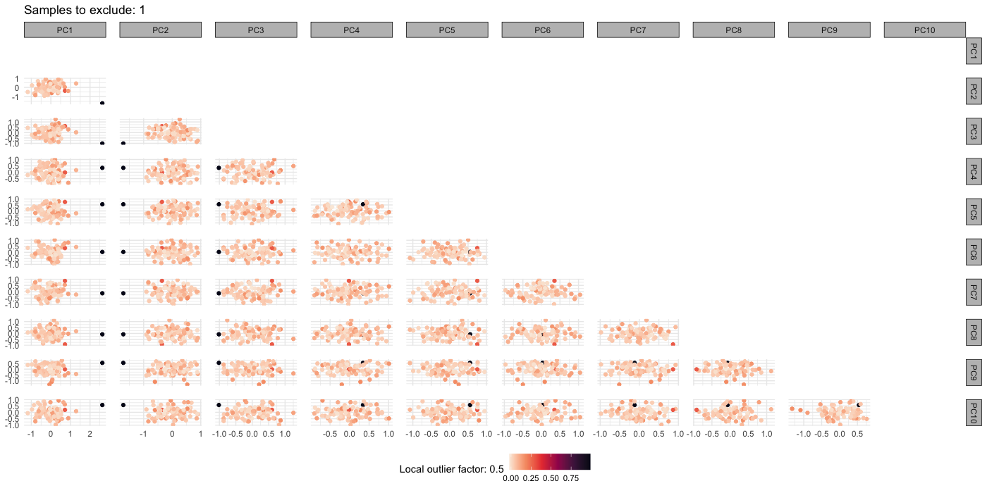

PCA + LOF outlier example

Plate correction

You can perform plate correction by providing sample and feature meta-data files.

data_processed <- process_data(
  data = data_features, 
  data_meta_samples = data_meta_samples,
  col_samples = "ID_sample", 
  data_meta_features = data_meta_features,
  col_features = "ID_feature",
  plate_correction = TRUE, 
  cols_listRandom = c("batch"), 
  cols_listFixedToKeep = c("age"), 
  cols_listFixedToRemove = c("sex"), 
  col_HeteroSked = NULL)

Other

Centering and scaling can be performed using centre_scale = TRUE. Centering and scaling is performed for log based transformations at the point of the transformation, regardless of if centre_scale = TRUE.

If you are processing case-control data then you will likely want to ensure excluded samples have their matched samples also excluded. This can be done using case_control = TRUE and providing the column name in data_meta_samples which has the matching factor, col_case_control = case_control_match.

The processed data, the IDs for excluded samples and features and the reasons for exclusions, and the outlier plot can be saved using save = TRUE and providing a file path for the processed data (path_out = path/to/directory/) and the exclusion data (path_outliers = path/to/directory/exclusions/)

References

Application of linear mixed models to remove unwanted variability (e.g., batch) and preserve biological variations while accounting for potential differences in the residual variances across studies (Viallon et al., 2021). The functions implementing this (normalization_residualMixedModels() and FUNnormalization_residualMixedModels()) utilise the R packages {pcpr2}, {lme4}, and {nlme}
- Viallon V, His M, Rinaldi S, et al. A New Pipeline for the Normalization and Pooling of Metabolomics Data. Metabolites. 2021;11(9):631. Published 2021 Sep 17. doi:10.3390/metabo11090631.
- {PCPR2}: Fages & Ferrari et al. (2014) Investigating sources of variability in metabolomic data in the EPIC study: the Principal Component Partial R-square (PC-PR2) method. Metabolomics 10(6): 1074-1083, doi: 10.1007/s11306-014-0647-9
- lme4: Bates, D., Mächler, M., Bolker, B., & Walker, S. (2015). Fitting Linear Mixed-Effects Models Using lme4. Journal of Statistical Software, 67(1), 1–48. doi.org/10.18637/jss.v067.i01.
- nlme: Pinheiro, J. C. & Bates, D. M. Mixed-Effects Models in S and S-PLUS. (Springer, New York, 2000). doi:10.1007/b98882
Sample exclusion performed using principal component analyses and a local outlier factor (Breuing et al., 2000) using a Tukey rule (Tueky, 1977) modified to account for skewness and multiple testing (Hubert and Vandervieren, 2008)
- Markus M. Breunig, Hans-Peter Kriegel, Raymond T. Ng, and Jörg Sander. 2000. LOF: identifying density-based local outliers. SIGMOD Rec. 29, 2 (June 2000), 93–104. doi.org/10.1145/335191.335388
- Tukey, J. W. Exploratory Data Analysis. (Addison-Wesley Publishing Company, 1977).
- Hubert, M. and Vandervieren, E., (2008), An adjusted boxplot for skewed distributions, Computational Statistics & Data Analysis, 52, issue 12, p. 5186-5201, EconPapers.repec.org/RePEc:eee:csdana:v:52:y:2008:i:12:p:5186-5201.
The implementation of sample exclusions is from the R package {bigutilsr} and is described in detail by Florian Privé in this blog post

The process_data() documentation

How